A brief tutorial on determining solid state diffusion coefficients with intermittent current interruption (ICI - a.k.a. 'fast GITT')

Introduction

Last year, my PhD student Yu-Chuan Chien, I, and other co-authors published a paper Rapid determination of solid-state diffusion coefficients in Li-based batteries via intermittent current interruption method in Nature Communications. This work was a development of my research on developing the intermittent current interruption (ICI) technique, in which we showed how we could use ICI to calculate ionic diffusion coefficients in battery materials as an alternative to the galvanostatic intermittent titration technique (GITT), but with a greatly reduced experimental time.

The paper has been out nearly a year now and has received good attention so far, with ~13k accesses at the journal, almost 30 citations and several people reaching out to us with questions. Some of those questions have been relating to the raw data archive at Zenodo, which was included as part of the supporting information. That archive contains all of the experimental data and code (written in R) that Yu-Chuan used to perform the data analysis. Unfortunately, though… updates to R and/or some of the add-on packages used in the code have meant that people cannot run the code in the Zenodo archive directly anymore and reproduce the analysis directly. That’s at least partly on us and something of a lesson learned in making longer-lived code archives.

Since most of the enquiries I have received have been from people interested to attempt the technique and the analysis themselves, I thought to try and put together a basic working example of the analysis and the calculations using one of the examples from the paper’s Zenodo archive. This example uses a more stripped-down, optimised version of the code that I use myself for doing ICI analysis. Generally, I recommend that anyone interested in using the technique on a regular basis invest some time into creating their own implementation of the analysis in whatever language they feel comfortable with.

Brief overview of the method

The ICI method itself is described in some detail already on this page. Essentially, we are performing a run-of-the-mill constant current cycling experiment on a coin-type lab battery cell and introducing short interruptions at regular intervals. In this case, the interruptions are 10 seconds in duration, every 5 minutes. We’re then analysing the potential or voltage change in that interruption to extract useful information about the resistance of the cell.

In this extended method, on top of the resistance parameters R and k we normally get, under certain circumstances we can calculate the solid state diffusion coefficient, according to the following formula:

\[D = \frac{4}{\pi} \left(\frac{V}{A} \frac{\frac{\Delta E_{OC}}{\Delta t_I}}{\frac{dE}{d\sqrt{t}}}\right)^2\]

For this we need the following quantities, two of which are variables which we will need to calculate from the experimental data:

\(\frac{V}{A}\): the ratio of the electrode volume to the surface area. In the original GITT paper, the electrodes were a solid metal foil, whereas here we are using porous electrodes. This introduces some complexity, but in this work we used the ratio of the specific volume (with units cm³ g^-1, obtained from XRD of the NMC811 material) with the specific surface area (with units cm² g^-1, obtained by BET). There are a few different ways to do this and this may not be the optimum, but it’s what we used.
\(\frac{\Delta E_{OC}}{\Delta t_I}\): the change in open circuit potential with respect to time. There are many ways to do this, and here I choose to calculate this using the E and t values from two data points from unique rest periods either side of the one I am calculating for. This means for a five-minute interruption, the quantity is calculated over a span of 20 minutes. It reduces ‘resolution’, but reduces the risk of error from noise. The current is also applied when these measurements are taken, so it is not a true open circuit potential, but the result is close enough for the purpose of this analysis.
\(\frac{dE}{d\sqrt{t}}\): this is the gradient of the E vs t^-1/2 regression for the current interruption, which is also used to calculate the k value.

Next, I’ll show an example of R code that can be used to do this calculation, and how to get it running.

Get started

For this, I’m using my M1 Macbook Pro with macOS 14 running a fairly recent version of R (4.3.1) with the tidyverse (2.0.0) package as the only key add-on package to worry about. The full output of sessionInfo() is at the bottom of this page.

The data I’ll be using for this can be downloaded here. You should find only two files: a text file containing the raw data, and an R script. The raw data is the same data for the operando XRD experiment published in the paper and in the original Zenodo archive, but I have stripped it down to only the essential columns, which are renamed for convenience. Bear in mind that this particular dataset is quite small, corresponding only to a partial cycle of the cell.

To load the tidyverse add-on package, set the working directory and import the data, we can do the following:

# Load the tidyverse package
library(tidyverse)

# Set working directory to location of files
setwd("path/to/downloaded/files")

df <- read_delim("chien_fastgitt_opxrd.txt")

Create a function, and use it

We should want to create a function to more easily handle different datasets which correspond to the same structure. The function below covers the complete transformation of the imported (and, note, already ‘cleaned’) data to a fully processed dataset containing all the quantities we want, ready for plotting. The function is organised into three major parts:

Add new columns for unique identifiers which will be useful for separating data later. I want the folowing variables: a unique column to indicate if the cell is charging, discharging or at rest; a unique identifier for each current on-off cycle; and a unique ‘step time’ for each step in the program, which is not included in the raw data.
Then, we need to split the data into two parts. In the output I want one ‘data point’ for each on-off cycle, but I need to analyse each current interruption to calculate the quantities I need. So, I’ll split a summary of the ‘current on’ part and the ‘current off’ parts into separate data frames and recombine them at the end.
The recombination itself, and here I can calculate most of the actual end results, such as the R, k and D values.

The code below is written to make use of the functions in the tidyverse ‘dplyr’ and ‘purrr’ packages for optimised efficiency and speed, so while some parts of this code may not be the easiest to read, it runs relatively fast. Trust me - for bigger datasets this is worthwhile!

# Define a function ici_example which performs the calculations required
ici_example <- function(df, tmin = 1, tmax = 10, V = 0.63056, A = 1.5E4) {

  # A new data frame 'sd' is created which adds the columns "state" (charge,
  # discharge, or 'R' (rest)), a unique counter variable 'rest', and step time.
  # It also modifies the charge variable so that the first Q value at the start
  # of each cycle is 0.
  sd <- df %>%
    # Now assign unique "state" (sign of current) and rest counter
    mutate(state = ifelse(I > 0, "charge", ifelse(I < 0, "discharge", "R")), 
           rest = imap(state, ~ ifelse(.x != "R" & state[.y-1] == "R", 1, 0)) %>%
             as.numeric %>%
             replace_na(0) %>%
             cumsum + 1
    ) %>%
    # Assign step time
    group_by(rest, state) %>%
    mutate(step.t = t - t[1]) %>%
    ungroup %>%
    # Reset charge to zero at start of each cycle.
    group_by(cyc.n) %>%
    mutate(Q = Q - Q[1]) %>%
    ungroup

  # If last charge-rest loop is not complete, it is removed, to avoid errors
  if (last(sd$state != "R")) {
    sd <- sd %>% filter(rest < max(rest))
  }

  # Collect data point for each individual rest
  # from each charge-rest loop, immediately before the rest. These values will
  # be the "t", "E", "Q" etc values recorded in the processed data.
  summary <- sd %>%
    group_by(rest) %>%
    filter(state != "R") %>%
    summarise_all(last)

  # For each rest cycle, a linear regression of E(we) vs t^1/2 is performed.
  # The intercept 'E0' and the gradient 's' are recorded, together with their
  # standard deviations
  regression <- sd %>%
    group_by(rest) %>%
    filter(state == "R", step.t >= tmin, step.t <= tmax) %>%
    group_modify(~ lm(E_p ~ sqrt(step.t), data = .x) %>%
                   with(
                     data.frame(
                       E0 = coef(summary(.))[1, 1],                
                       E0_err = coef(summary(.))[1, 2], #and error
                       s = coef(summary(.))[2, 1], #and gradient
                       s_err = coef(summary(.))[2, 2] #and error
                     )))

  # The output data frame is produced by combining the summary and regression
  # data frames, and the quantities R, k, dE/dt and D are calculated.
  out <- Reduce(function(x, y) merge(x, y, by = "rest"), 
                list(summary, regression)) %>%
   mutate(R = (E - E0) / (I / 1000), R_err = E0_err / (abs(I) / 1000),
           k = -1 * s / (I / 1000), k_err = s_err / (abs(I) / 1000),
           dEdt = (E-lag(E, 2))/(t-lag(t, 2)),
          D = (4/pi) * ((V/A) * (dEdt/s))^2
    )

  # The output data frame is returned.
  return(out)

}

To use this function itself is then very straightforward. Note that the default arguments include the specific values of V and A for the calculation, which you would probably not do in practice:

# The processed data is called by using the function ici_example on the
# data frame df with the default arguments.
processed <- ici_example(df)

Plot!

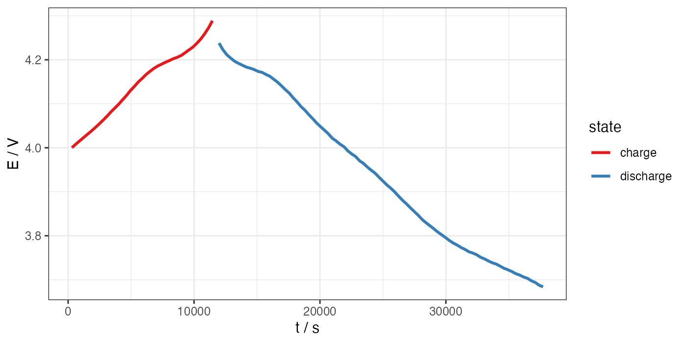
Now, we can start making some plots. Again, bear in mind that this particular example dataset represents only a partial cycle of the cell.

# ggplot for E vs t
ggplot(processed, aes(x = t, y = E)) +
  geom_path(aes(color = state), size = 1) +
  theme_bw() +
  scale_color_brewer(palette = "Set1") +
  labs(x = "t / s", y = "E / V")

ggsave("E-t.png", width = 7, height = 3.5, units = "in", dpi = 200)

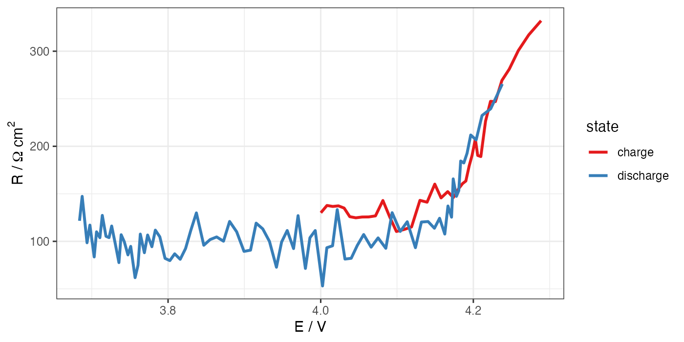
Electrode potential (E) vs time (t), output from the above code

# ggplot for R vs E
ggplot(processed, aes(x = E, y = R * 1.327)) +
  geom_path(aes(color = state), size = 1) +
  theme_bw() +
  scale_color_brewer(palette = "Set1") +
  labs(x = "E / V", y = "R /"~Omega~"cm"^"2")

ggsave("R-E.png", width = 7, height = 3.5, units = "in", dpi = 200)

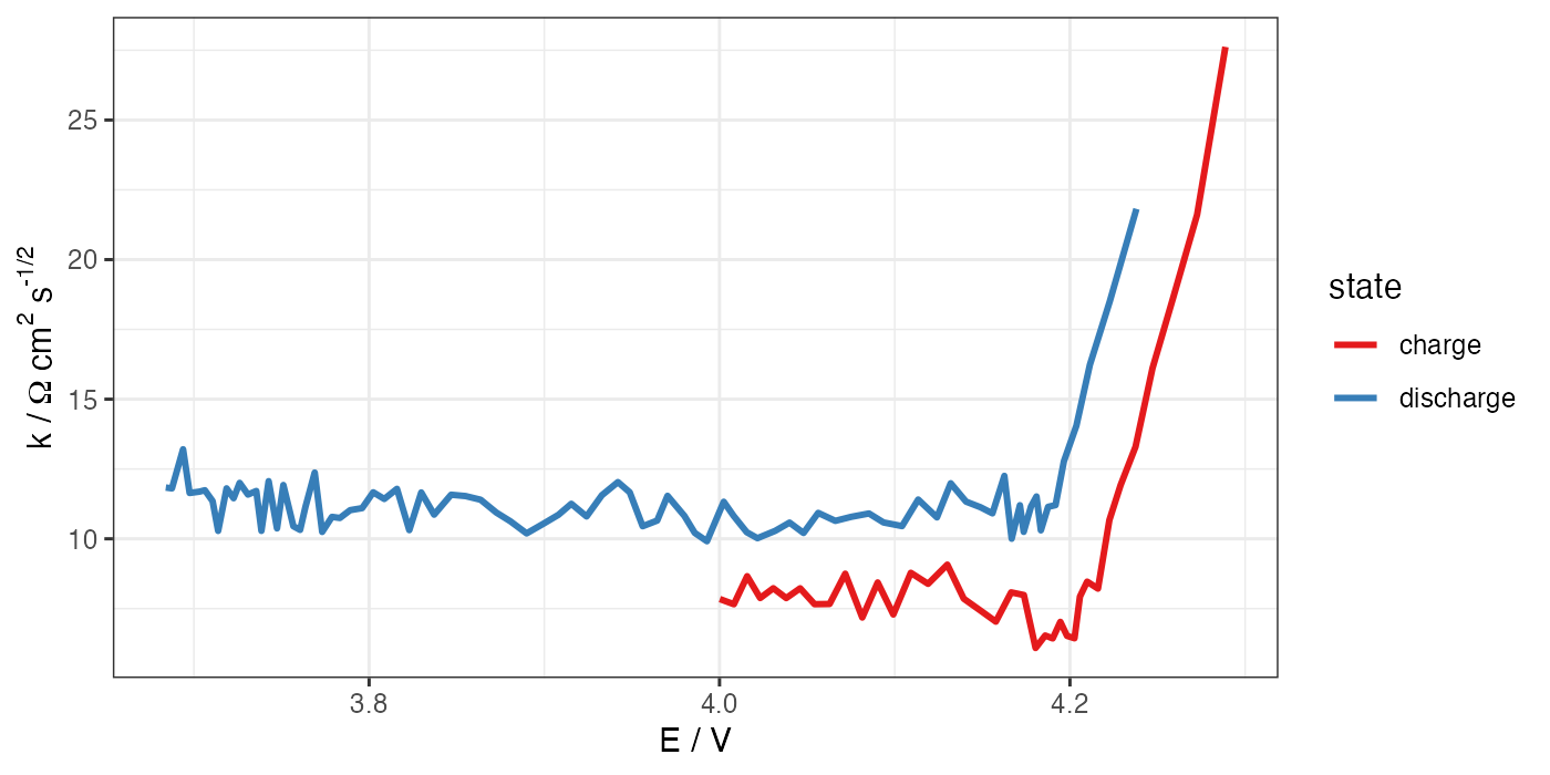
Areal resistance (R) vs electrode potential (E), output from the above code

# ggplot for k vs E
ggplot(processed, aes(x = E, y = k * 1.327)) +
  geom_path(aes(color = state), size = 1) +
  theme_bw() +
  scale_color_brewer(palette = "Set1") +
  labs(x = "E / V", y = "k /"~Omega~"cm"^2~"s"^"-1/2")

ggsave("k-E.png", width = 7, height = 3.5, units = "in", dpi = 200)

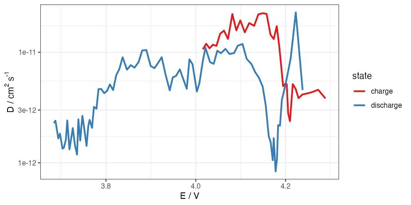
Areal diffusion resistance coefficient (k) vs electrode potential (E), output from the above code

# ggplot for D (log scale) vs E
ggplot(processed, aes(x = E, y = D)) +
  geom_path(aes(color = state), size = 1) +
  theme_bw() +
  scale_color_brewer(palette = "Set1") +
  scale_y_log10() +
  labs(x = "E / V", y = "D / cm"^"2"~"s"^"-1")

ggsave("D-E.png", width = 7, height = 3.5, units = "in", dpi = 200)

Diffusion coefficient (D) vs electrode potential (E), output from the above code

Parting words

As mentioned above, I think it is beneficial for anyone interested in using this technique to make the effort to develop their own implementation of the code. I understand not that many people in the field are R users, but I’m perfectly happy for this code to be copied and adapted as necessary. It has been fairly carefully refined over the years and I think works quite well, if a bit lacking in error handling.

The main thing I would wish to caution any users would be that the experimental part of this technique is just as important, if not more so, than the data analysis. GITT is notorious for resulting in order-of-magnitude errors if the assumptions are not met, and this applies to the analysis here as well, since it’s derived under the same principles.

In this particular experiment, we did a few things to try and minimise the deviation from ideal behaviour, e.g.:

Thin electrode, to minimise the influence of electrolyte diffusion in the composite electrode
Single crystal NMC material with relatively narrow particle size distribution, to narrow the distribution of diffusion time constants
Low current, to reduce the effect of IR drop
Three-electrode cell, to mitigate the influence of a Li metal (or any other) counter electrode

I also recommend readers to look at this paper with Zeyang Geng as first author, which I consider to be a sister paper to the experimental paper, and which deals with the calculation of diffusion coefficients from GITT and ICI on a more theoretical basis. In particular, in that paper we simulated GITT and ICI experiments with a Doyle-Fuller-Newman model of a cell with a known solid state diffusion coefficient, and tried to back-calculate it - and we don’t get the same number! So, to conclude - try the method out, but use with care!

Output of `sessionInfo()`:

R version 4.3.1 (2023-06-16)
Platform: aarch64-apple-darwin20 (64-bit)
Running under: macOS Sonoma 14.1.1

Matrix products: default
BLAS:   /System/Library/Frameworks/Accelerate.framework/Versions/A/Frameworks/vecLib.framework/Versions/A/libBLAS.dylib 
LAPACK: /Library/Frameworks/R.framework/Versions/4.3-arm64/Resources/lib/libRlapack.dylib;  LAPACK version 3.11.0

locale:
[1] en_US.UTF-8/en_US.UTF-8/en_US.UTF-8/C/en_US.UTF-8/en_US.UTF-8

time zone: Europe/Stockholm
tzcode source: internal

attached base packages:
[1] stats     graphics  grDevices utils     datasets  methods   base     

other attached packages:
 [1] lubridate_1.9.2 forcats_1.0.0   stringr_1.5.0   dplyr_1.1.2     purrr_1.0.1     readr_2.1.4    
 [7] tidyr_1.3.0     tibble_3.2.1    ggplot2_3.4.2   tidyverse_2.0.0

loaded via a namespace (and not attached):
 [1] bit_4.0.5          gtable_0.3.3       crayon_1.5.2       compiler_4.3.1     tidyselect_1.2.0  
 [6] blob_1.2.4         parallel_4.3.1     textshaping_0.3.6  systemfonts_1.0.4  scales_1.2.1      
[11] fastmap_1.1.1      R6_2.5.1           labeling_0.4.2     generics_0.1.3     munsell_0.5.0     
[16] DBI_1.1.3          RColorBrewer_1.1-3 pillar_1.9.0       tzdb_0.4.0         rlang_1.1.1       
[21] utf8_1.2.3         cachem_1.0.8       stringi_1.7.12     bit64_4.0.5        timechange_0.2.0  
[26] RSQLite_2.3.1      memoise_2.0.1      cli_3.6.1          withr_2.5.0        magrittr_2.0.3    
[31] grid_4.3.1         vroom_1.6.3        rstudioapi_0.15.0  hms_1.1.3          lifecycle_1.0.3   
[36] vctrs_0.6.3        glue_1.6.2         farver_2.1.1       ragg_1.2.5         fansi_1.0.4       
[41] colorspace_2.1-0   tools_4.3.1        pkgconfig_2.0.3

On This Page

A brief tutorial on determining solid state diffusion coefficients with intermittent current interruption (ICI - a.k.a. 'fast GITT')

On This Page

Introduction

Brief overview of the method

Get started

Create a function, and use it

Plot!

Parting words

Output of `sessionInfo()`:

On This Page

A brief tutorial on determining solid state diffusion coefficients with intermittent current interruption (ICI - a.k.a. 'fast GITT')

On This Page

Introduction

Brief overview of the method

Get started

Create a function, and use it

Plot!

Parting words

Output of sessionInfo():

Output of `sessionInfo()`: