impedanceR - an R package for simulating impedance spectra of equivalent circuits

Introduction

This package contains a suite of functions for calculating and simulating electrical or electrochemical impedance spectra using the R programming language. The package contains functions for simulating the most common equivalent circuit elements, some convenient functions for constructing the circuits themselves, and other useful utility functions.

I used early versions of this code throughout my introduction to EIS pages to simulate equivalent circuits and create the interactive components of those pages.

For those interested, I have now released this code as a more convenient R package on GitHub, which also contains some improved functionality and additional equivalent circuit elements. This page gives some basic instructions on installation and usage.

Installation

You will need R and the devtools package installed. I also recommend RStudio and the tidyverse suite of add-on packages for working with data - I will use this in my examples. (The impedanceR package also requires magrittr which provides the pipe (%>%) operator).

devtools::install_github("mjlacey/impedanceR")
library(impedanceR)

Functions provided

You can consult the R documentation (i.e., by using ?functionname) for more information on each specific function.

Equivalent circuit elements

The following equivalent circuit elements and the arguments (i.e., parameters they take) are as follows:

Z_R(R) - resistor

Z_C(C, omega) - capacitor

Z_L(L, omega) - inductor

Z_Q(L, n, omega) - constant phase element

Z_W(sigma, omega) - Warburg element

Z_FLW(Z0, tau, omega) - Finite Length (“short”) Warburg element (FLW)

Z_FSW(Z0, tau, omega) - Finite Space (“open”) Warburg element (FSW)

Z_G(Z0, k, omega) - Infinite length Gerischer element

Z_FLG(Z0, k, tau, omega) - Finite length Gerischer element

trans_line(R, U, n) - transmission line

Other functions

para() - for adding any number of circuit elements in parallel

omega_range() - for calculating a range of angular frequency values (necessary for all circuit elements, except resistors)

Z_to_df() - convert a complex vector to a data.frame of real and imaginary values

Basic usage

All of the equivalent circuit elements (except the resistor) take a vector of angular frequency values (omega, that is, the frequency data points to be simulated) as an argument, and all output a vector of complex numbers as a result.

All the elements in the circuit need to use the same omega values, so it is simplest to define these as its own variable at the start, using the omega_range function:

omega = omega_range(low.logf = 0, high.logf = 5, p.per.dec = 12)

This creates a set of values for angular frequency from 1 Hz to 10 kHz, with 12 points per decade of frequency.

Equivalent circuits can be calculated by mathematically adding them in series (with the + operator) or in parallel (with the provided para() function). Let’s consider a circuit with two parallel RC elements in series with each other:

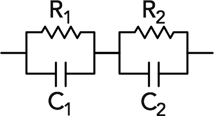
a <- para(Z_R(5), Z_C(1E-5, omega)) +
 para(Z_R(20), Z_C(1E-4, omega))

We can check that the variable a has the right form:

str(a)

cplx [1:61] 25-0.3i 25-0.3i 25-0.4i ...

And this is the expected result - a vector of complex numbers. The provided Z_to_df() function converts this to a data frame:

a %>%
  Z_to_df() %>%
  head

  Re       Im
1 24.99684 -0.2528585
2 24.99536 -0.3063226
3 24.99320 -0.3710783
4 24.99002 -0.4495006
5 24.98535 -0.5444561

And we can plot this (using, by convention, the negative imaginary part). If using ggplot2, use the coord_fixed() option to make sure that the axes are proportional!

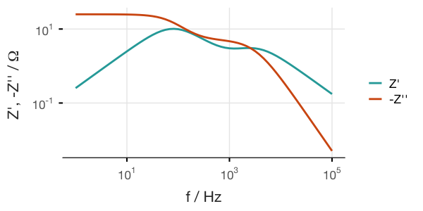
We can also create Bode plots, but this requires adding the omega variable (or frequency, which is omega divided by 2π) to the data frame. I find the easiest way is to use gather() from the dplyr package:

a %>% Z_to_df() %>%
  mutate(f = omega / (2 * pi), Im = -Im) %>%
  gather(key = key, value = value, -f) %>%
  ggplot(aes(x = f, y = value)) +
  geom_path(aes(color = key), size = 1) +
  scale_x_log10(labels=trans_format('log10',math_format(10^.x))) +
  scale_y_log10(labels=trans_format('log10',math_format(10^.x)))

and so forth.

Transmission lines

One feature I will highlight in particular is the possibility to simulate transmission line style circuits, which are useful for example in modelling porous electrodes.

The basic function trans_line() takes the form:

trans_line(R, U, n)

where in the equivalent circuit below, R is the value of each individual resistor in one of the rails of the transmission line, U is any other equivalent circuit unit which shorts the two rails together, and n is the total number of R-U units linked together. The opposite rail has zero resistance (this is a limitation currently, I’m afraid).

So for example, we can simulate the classic de Levie transmission line as discussed in my page on diffusion resistance, where U is just a capacitor:

b <- trans_line(R = 2, U = Z_C(1E-6, omega), n = 40)

So now we are calculating the impedance of a transmission line where each resistor has a value of 2 Ω, the U unit is a capacitor with a capacitance of 1 µF, and the total transmission line is 40 units long. If we plot this, we get:

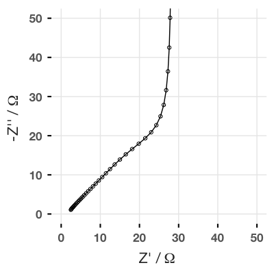
And this result has the same shape as the finite space Warburg (FSW) element, where the Z₀ parameter is equal to the sum of all the resistors in the rail.

Here’s a more complicated example. Let’s imagine a more complicated model where the U unit in the transmission line is a modified Randles circuit (this is the sort of thing we might consider as a model for a battery electrode, for example). In 13 lines, I can simulate this equivalent circuit for several different lengths of transmission line, and make a basic plot of the data.

omega <- omega_range(-1, 5, 12)

lapply(c(5, 10, 20, 40), function(n) {
  res <- trans_line(R = 2,
                    U = para(Z_R(10), Z_C(1E-7, omega)) +
                      para(Z_C(1E-6, omega), Z_R(15) + Z_FSW(100, 0.5, omega)),
                    n = n)
  res %<>% Z_to_df %>%
    mutate(n = factor(n))
}) %>%
  do.call(rbind, .) %>%
  ggplot(aes(x = Re, y = -Im)) +
  geom_path(aes(color = n), size = 1) +
  coord_fixed(ylim = c(0, 20)) +
  labs(x = "Z' /"~Omega~"", y = "-Z'' /"~Omega~"")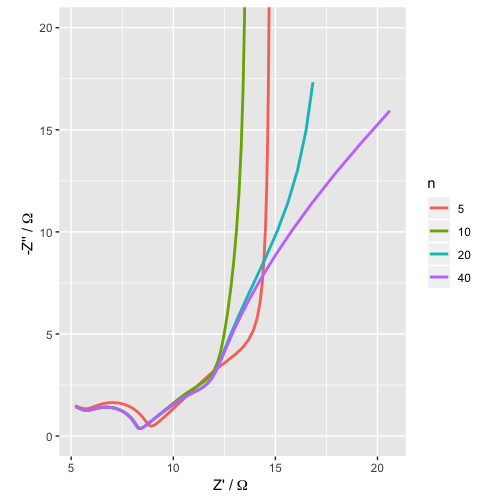

Give it a try! Any questions, feel free to contact me or ask in the comments below.